LEARN HOW TO CREATE AUTOMATIC
ATTENDANCE SHEET IN MS-EXCEL:
- Automatic attendance sheet system can help any school, college , or any organisation in most of the way.
WHAT IS MICROSOFT EXCEL:
- MS-Excel is a program that is having a collection of cells arranged into row and column to organize , format and calculate data with some formula that are also inbuilt in excel , and is having a spreadsheet system.
WHAT ARE THE USES OF MS -EXCEL :
MS-EXCEL is the very powerful tool , today. It is almost used in every organisation for some purposes.
- Excel is a powerful tool for data entry work, it can store a large number of data. Here we can create a data entry form as per the business needs.
- It can be used to maintain employee details.
- Excel has some accounting templates for easy use , formulas that are inbuilt in it help us to organize and synthesize the results.
- It can also be used to check duplicate entries .
- It helps us to build great charts.
- Excel also offers some tools that allow user to create flowcharts, which can consist of text, images, and animation.
- It uses for collection and verification work .
- Use for data filtering.
- It can perform many mathematical calculations also .
- Most interesting about excel is that we can automate the reports in excel by using VBA coding language.
WHAT IS USE OF AUTOMATIC ATTENDANCE SHEET :
- Automatic attendance sheet system can help any school, college , or any organisation in most of the way.
- It help in saving both money and time as it remove manual process of calculating some entries , automatic attendance sheet in excel reduces paperwork.
- Eliminate any duplicate entries and any errors.
- MS -Excel automatic attendance sheet system can manage student attendance and absenteeism records.
- This system can manage the records of teachers, any staff , assign workers etc.
STEPS TO CREATE / GENERATE
AUTOMATIC ATTENDANCE SHEET
USING MS-EXCEL:
1 .Before creating attendance sheet , first learn this term D11 OR E12 what are they what they indicate before going further .
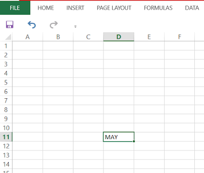
- D11 here means that we have written may in a cell which is in the D column and at the 11 number from top cell. so the position of text "may" is D11 here. .
- You will see these names like D11 , g12 etc in the formulas.
In any formula if you want to write a position of any cell, just click on that cell .
2. Second learn how to create drop down list in excel:
This GIF below is showing , how we create any drop down list in MS - excel.
Now you are ready to learn how to create automatic attendance sheet in ms excel Now we are going to learn step by step how to create an automatic attendance sheet in Microsoft excel.
STEP :1 First open the Microsoft excel in your PC or laptop. Take two sheets, sheet 1 and sheet 2. In the sheet 1 write attendance sheet for month in the cell as shown in below figure.
STEP :2 Now go to sheet -2 , write there JAN in any cell , then drag that cell up to DEC .After completing this list from Jan to Dec, go back to sheet 1.
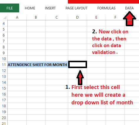
STEP :3 Now in the sheet 1 select that cell where you want to create drop down list of the month , after that click on data at top bar , then click on data validation option under this data option.Look at the image below :
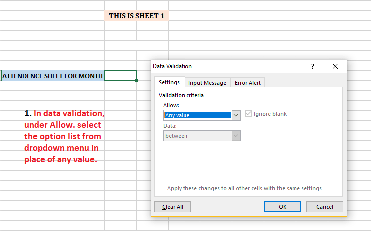
STEP :4 Now in allow drop down box , select option "list".
STEP :5 After selecting list option , Put your cursor in source text box , then go to sheet 2 then select the cells range from Jan to Dec and then click ok.
STEP :6 Now drop down list will be created like this as shown below in the picture in sheet 1 .
STEP:7 Now in sheet 1 create first date and last date column as shown in the image below , and let me select month "may " from drop down list of month, you can select any month i am taking the example with "may" month. The blank cell corresponding to first and last date here we will add formulas.
STEP:8 Write the formula corresponding to first date cell.
=datevalue("1"& Position of may cell) , then press enter. You will get 1-05-20 as the first date.
You can change the format of date by right click---then click on format cell --then choose date Here in this image shown below D11 is the position of the cell where we have written"may".
STEP:9 Now write formula in the last date cell.
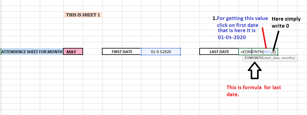
=EOMONTH(click on position of first date that we have just created , 0). press enter , now you will get 31-05-20 written there in last date .
Here in the image below H11 , in the formula is the position of the first date cell where 1-05-20 is written .
STEP:10 Now create name column , date and days rows , as shown in the image below ,for getting your first date there just write formula
=then click on 01-05-20 written corresponding to the first date .
You will get this view now
STEP:11 Now for getting second date of may write formula over there :
=if(position of 1-05-20<position of 31-05-20 , position of 1-05-20 + 1, "").
After writing formula press enter then you will get 2-05-20 written over there,Now drag this date , until the date of end date of month.
In the image below in formula : H11 is the position of 1-05-20 here
M11 is the position of 31-05-20
" " indicate otherwise null value
 |
| STEP:11 |
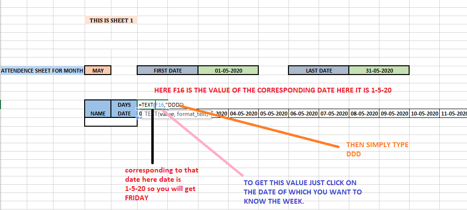
STEP 12: Now we will write formula in the day row , such that it will automatically gives us the day that was on ,that corresponding date. now this formula will write the day automatically that was on 01-05-20.
=Text(position of the cell corresponding to which you want the day ,"DDD")
In the picture below F16 is position of date 01-05-20.
STEP:13 Now drag the this cell , to get all the days corresponding to each date , have a look in this picture below.
STEP:14 Now we will check if we change the month from may to June , then also we are getting correct days corresponding to every date or not .
Now select month June , then see the date and days have changed according to month June, here it is showing on 1 June --- Monday, and it is right on 1-June-20 it was Monday.
STEP:15 Now i want to highlight all Sunday with red color, like the way if i will change month in every month Sunday should be highlighted.
- Now select the cell under the Sunday .
- Now go to home, select conditional formatting.
- Then click on the option -- use a formula to determine which cell to format .
- Now write formula in the edit rule Text box : =OR(click on sun ='sun').
- Now click on format---fill ---select color---click ok.
In the figure H$15 is position of Sun here.
STEP:16 Now sun will be highlighted ,now just click on format then select the rows and column that you want to format , now all the Sundays will be highlighted like this.
STEP:17 Now we will do formatting of text i want if i write P here represent present in the cell then it should be automatically turns green, if i write A (absent) in any cell then it should automatically fill with red color .
For this go to home ----click on conditional formatting -----click on highlight cell rule -----click on text that contain.
Now pop up will appear here write P in the text box and select color from drop down option .
Now again repeat same process now write A in text box and select the color .
 |
| STEP:17 |
STEP:18 Now you will get the sheet like this as shown below.
- Now your attendance sheet is ready.
- You can also add some more feature in it, like you can add one column of that will give you the count of number of days any person was absent just by writing formula of =count , in that cell .
- Employee of the organisation can do some more text like paid leave , causal leave and can do formatting like we have done of P and A . Then he can also add some extra column which will give the count of its causal leave or paid leave of each month automatically .You can modify it as your requirements , it is just a one sample of how automatic attendance sheet can be created.
WATCH THIS GIF GIVEN BELOW:
This GIF below will show you how your final automatic attendance sheet will look and how it will work.
Here this attendance sheet is having some extra column SL, CL, and sum. sum column will give the sum of both sick leave (SL) and causal leave (CL). column SL will contain count of all sl leave and Cl column will contain count of all cl leave.This has been done by using count and sum formula in excel.
Whenever i will write p in any cell it will be automatically highlighted with green and whenever i will write sl or cl it will be highlighted with yellow .
Then finally Sl column will give us the number of sick leave of may month.Cl column will give us the number of causal leave OF may month. sum column will give the sum of both sl and cl leave .
HAVE A LOOK BELOW ON THE GIF, TO SEE FINAL AUTOMATIC ATTENDANCE SHEET IN EXCEL:








Comments
Post a Comment